From Reinforcement Learning to Generalised Bayesian Filtering#
![]()
Show code cell content
import sys
from IPython.utils import io
if 'google.colab' in sys.modules:

  with io.capture_output() as captured:
      ! pip install pyhgf watermark
import jax.numpy as jnp
import matplotlib.pyplot as plt
import numpy as np
import seaborn as sns
from matplotlib.ticker import MultipleLocator
from pyhgf.math import MultivariateNormal, Normal, gaussian_predictive_distribution
from pyhgf.model import Network
from pyhgf.utils import beliefs_propagation
from scipy.stats import norm, t

np.random.seed(123)
plt.rcParams["figure.constrained_layout.use"] = True
Hierarchical Gaussian filters can receive one-dimensional continuous and binary inputs by default, but they in practice be extended to a much broader class of distributions. Here, we use the approach described in [Mathys and Weber, 2020] to demonstrate that the Hierarchical Gaussian Filter can be generalized to any probability distribution that belongs to the exponential family. This is the sample principle that underpins the The categorical Hierarchical Gaussian Filter, in which case the implied distribution is a Dirichlet distribution. However, by abstracting the specificity of each distribution away, we can implement probabilistic nodes that can flexibly filter any distribution from the exponential family, as an input node or as a state node, which greatly enlarges the range of possible models.
Generalised Bayesian filtering in this context requires first expressing the Bayesian update of an exponential family distribution as a simple update over hyperparameters. Exponential families of probability distributions are those which can be written in the form:
where:
\(x\) is a vector-valued observation
\(\vartheta\) is a parameter vector
\(h(x)\) is a normalization constant
\(\eta(\vartheta)\) is the natural parameter vector
\(t(x)\) is the sufficient statistic vector
\(b(\vartheta)\) is a scalar function
It has been shown in [Mathys and Weber, 2020] that, when chosing as prior:
with the variable
as normalization constant, then the posterior is a simple update of the hyperparameters in the form:
Filtering the Sufficient Statistics of a Stationary Distribution#
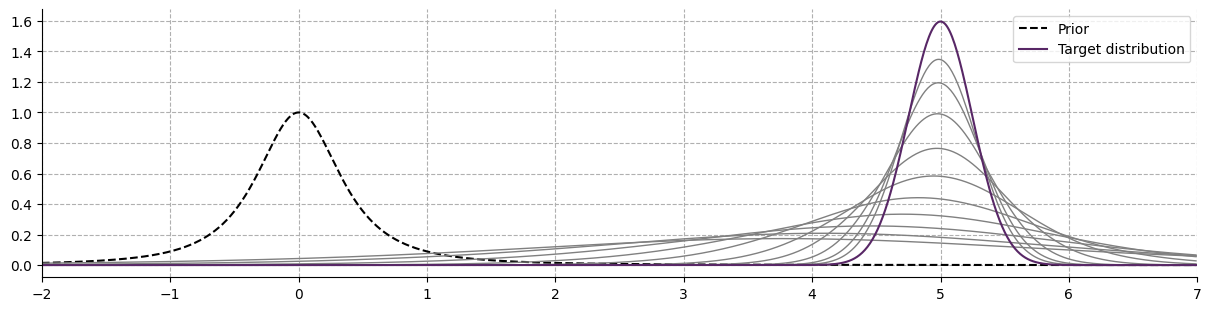
We start applying this update steps to the estimation of the parameters from a stationary normal distribution.
x = np.arange(-7, 7, 0.01)  # x axis
xi, nu = np.array([0, 1 / 8]), 1.0  # initial hyperparameters
xs = np.random.normal(5, 1 / 4, 1000)  # input observations
plt.figure(figsize=(12, 3))
plt.plot(
    x,
    gaussian_predictive_distribution(x, xi=xi, nu=nu),
    color="k",
    label="Prior",
    linestyle="--",
)
for i, x_i in enumerate(xs):
    xi = xi + (1 / (1 + nu)) * (Normal().sufficient_statistics(x=x_i) - xi)
    nu += 1

    if i in [2, 4, 8, 16, 32, 64, 128, 256, 512, 999]:
        plt.plot(
            x,
            gaussian_predictive_distribution(x, xi=xi, nu=nu),
            color="grey",
            linewidth=1.0,
        )
plt.plot(
    x, norm.pdf(x, loc=5.0, scale=1 / 4), color="#582766", label="Target distribution"
)
plt.xlim(-2, 7)
plt.legend()
plt.grid(linestyle="--")
sns.despine()
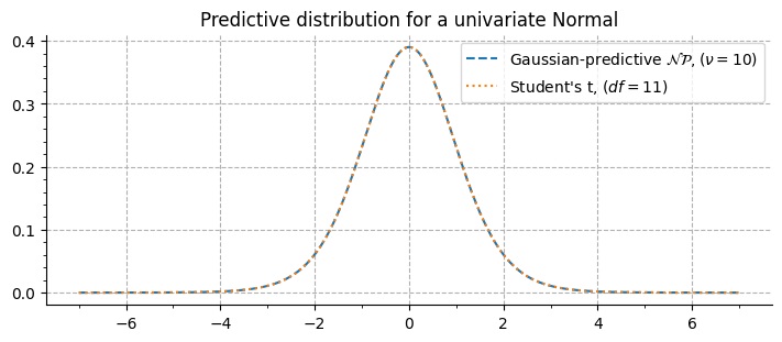
The vizualisation of the predictive distribution over new observations require integrating the joint probability of the prior \(g_{\xi, \nu}(\vartheta)\) and the posterior \(f_x(\vartheta)\). In the case of a univariate normal, the Gaussian-predictive distribution is given by:
When \(\xi = 0, 1\), this corresponds to the Student’s-t distribution with \(\nu + 1\) degrees of freedom, as evidenced here:
Show code cell source
_, ax = plt.subplots(figsize=(7, 3))
ax.plot(
    x,
    gaussian_predictive_distribution(x, xi=np.array([0, 1]), nu=10),
    linestyle="--",
    label=r"Gaussian-predictive $\mathcal{NP}, (\nu = 10)$",
)

ax.plot(x, t.pdf(x, 11), linestyle=":", label=r"Student's t, $(df = 11)$")
ax.xaxis.set_minor_locator(MultipleLocator(1))
ax.yaxis.set_minor_locator(MultipleLocator(0.02))
ax.set_title("Predictive distribution for a univariate Normal")
ax.legend()
ax.grid(linestyle="--")
sns.despine()
Filtering the Sufficient Statistics of a Non-Stationary Distribution#
Real-world applications of Bayesian filtering imply non-stationary distributions, in which cases the agent cannot rely anymore on distant observation and has to weigh down their evidence proportional to their distance from the current time point. In the current framework, this suggests that \(\nu\), the pseudo-count vector, cannot linearly increase with the number of new observations but has to be limited. The most straightforward way is then to fix it to some values.
Using a fixed \(\nu\)#
This operation can be achieved using a continuous state node that implements the exponential family updates on the values that are passed by the value child nodes. Such nodes are referred to as ef- nodes, with the type of distribution (here a simple one-dimensional Gaussian distribution, therefore the kind is set to "ef-normal"). The input node is set to generic, which means that this input simply passes the observed value to the value parents without any additional computation. We can define such a model as follows:
generalised_filter = (
    Network()
    .add_nodes(kind="generic-state")
    .add_nodes(kind="ef-normal", value_children=0, xis=np.array([0, 1 / 8]))
)
generalised_filter.plot_network()

We then create a time series to filter and pass it to the network using different values for the parameter \(\nu\), representing how much past values should influence the Bayesian update.
x = np.arange(0, 1000)  # time points

# create noisy input time series with switching means
xs = np.random.normal(0, 1 / 8, 1000)
xs[200:400] += 0.5
xs[600:800] -= 0.5
means = []
nus = [3, 9, 35]
for nu in nus:
    # set the learning rate
    generalised_filter.attributes[1]["nus"] = nu

    means.append(generalised_filter.input_data(input_data=xs).to_pandas().x_1_xis_0)
Show code cell source
_, ax = plt.subplots(figsize=(12, 3))
ax.scatter(x, xs, color="grey", alpha=0.6, s=10)
for mean, nu in zip(means, nus):
    ax.plot(x, mean, label=rf"$\nu = {nu}$")
ax.grid(linestyle="--")
ax.set_title(r"Filtering sufficient statistics using a fixed $\nu$")
ax.set_xlabel("Observations")
ax.legend()
sns.despine()
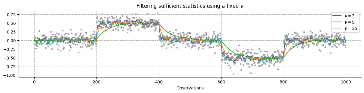
We can see that larger values for \(\nu\) correspond to a lower learning rate, and therefore smoother transition between states.
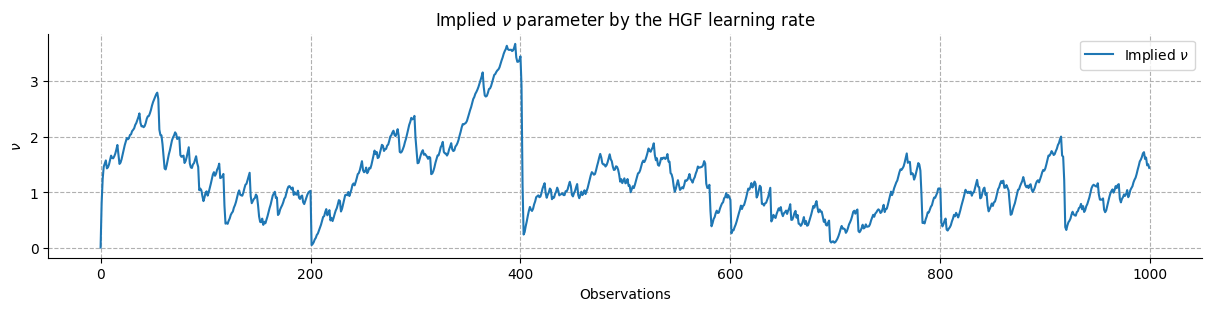
Using a dynamically adapted \(\nu\) through a collection of Hierarchical Gaussian Filters#
Limiting the number of past observations weighting in the predictive distribution comes with the difficult question of how to choose the correct value for such a parameter. Here, one solution to handle this is to let this parameter vary across time as a function of the volatility of the observations. Large unexpected variations should increase the learning rate, while limited, expected variations should increase the posterior precision. Interestingly, this is the kind of dynamic adaptation that reinforcement learning models are implementing, including the Hierarchical Gaussian Filter in this category. Here, we can derive the implied \(\nu\) from a ratio of prediction and observation differentials such as:
with \(\delta\) the prediction error at time \(k\) and \(\Delta\) the differential of expectations (before and after observing the new value).
Univariate normal distribution#
univariate_hgf = (
    Network()
    .add_nodes(node_parameters={"precision": 100})
    .add_nodes(value_children=0, node_parameters={"tonic_volatility": -6.0})
    .add_nodes(
        volatility_children=[1], node_parameters={"mean": 0, "tonic_volatility": -2}
    )
)
attributes, edges, update_sequence = univariate_hgf.get_network()

nus = []
for i, x_i in enumerate(xs):
    mean = attributes[1]["mean"]

    attributes, _ = beliefs_propagation(
        edges=edges,
        attributes=attributes,
        inputs=(x_i, 1, 1.0),
        update_sequence=update_sequence,
        input_idxs=univariate_hgf.input_idxs
    )

    new_mean = attributes[1]["mean"]

    nus.append(((x_i - mean) / (new_mean - mean)) - 1)
_, ax = plt.subplots(figsize=(12, 3))
ax.plot(x, nus, label=rf"Implied $\nu$")
ax.grid(linestyle="--")
ax.set_title(r"Implied $\nu$ parameter by the HGF learning rate")
ax.set_ylabel(r"$\nu$")
ax.set_xlabel("Observations")
ax.legend()
sns.despine()
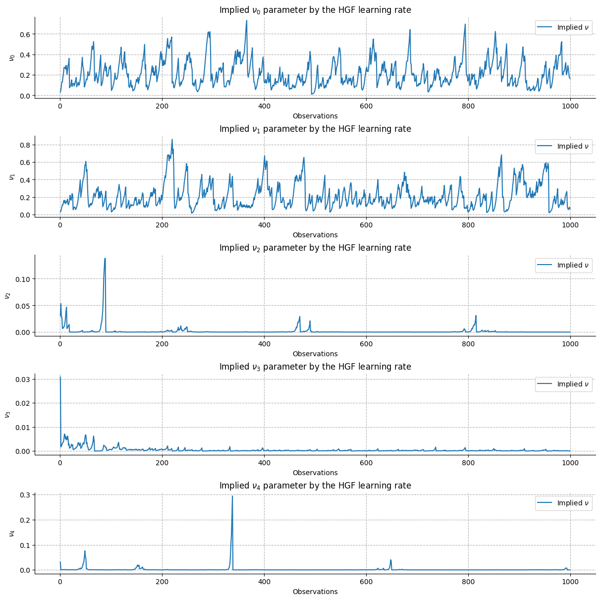
Bivariate normal distribution#
# simulate an ordered spiral data set
N = 1000
theta = np.sort(np.sqrt(np.random.rand(N)) * 5 * np.pi)
r_a = -2 * theta - np.pi
input_data = np.array([np.cos(theta) * r_a, np.sin(theta) * r_a]).T
input_data = input_data + np.random.randn(N, 2) * 2
# get the sufficient statistics from the first observation to parametrize the model
sufficient_statistics = jnp.apply_along_axis(
    MultivariateNormal().sufficient_statistics, 1, input_data
)
Filtering the sufficient statistics of a two dimensional multivariate normal distribution requires tracking the values of 5 parameters in paralell. Our model therefore consist in 5 independent two-level continuous HGF.
bivariate_hgf = Network().add_nodes(node_parameters={"recision": 0.1}, n_nodes=5)

for i in range(5):
    bivariate_hgf.add_nodes(
        value_children=i,
        node_parameters={
            "tonic_volatility": -6.0,
            "mean": sufficient_statistics[0][i],
        },
    )

for i in range(5):
    bivariate_hgf.add_nodes(
        volatility_children=[i + 5],
        node_parameters={"mean": 10.0, "tonic_volatility": -2},
    )
bivariate_hgf.plot_network()

For us to compute the hyperparameter after each update, we need to manually call the belief propagation sequence.
attributes, edges, update_sequence = bivariate_hgf.get_network()

nus, means = [], []
for i in range(input_data.shape[0]):
    mean = jnp.array([attributes[i]["mean"] for i in range(5, 10)])
    means.append(mean)

    # interleave observations and masks
    data = tuple(np.column_stack((sufficient_statistics[i], np.ones(sufficient_statistics[i].shape, dtype=int))).ravel())

    attributes, _ = beliefs_propagation(
        edges=edges,
        attributes=attributes,
        inputs=(*data, 1.0),
        update_sequence=update_sequence,
        input_idxs=bivariate_hgf.input_idxs
    )

    new_mean = jnp.array([attributes[i]["mean"] for i in range(5, 10)])
    nus.append(((sufficient_statistics[i] - mean) / (new_mean - mean)) - 1)
nus = jnp.array(nus)
means = jnp.array(means)
Show code cell source
_, ax = plt.subplots(figsize=(12, 12), nrows=5)
for i in range(5):
    ax[i].plot(x, nus[:, i], label=rf"Implied $\nu$")
    ax[i].grid(linestyle="--")
    ax[i].set_title(rf"Implied $\nu_{i}$ parameter by the HGF learning rate")
    ax[i].set_ylabel(rf"$\nu_{i}$")
    ax[i].set_xlabel("Observations")
    ax[i].legend()
sns.despine()
Show code cell content
# run this code to create the animation

# fig, ax = plt.subplots(figsize=(5, 5))
# scat = ax.scatter(
#     input_data[0, 0],
#     input_data[0, 1],
#     edgecolor="k",
#     alpha=0.4,
#     s=10
# )
# scat2 = ax.scatter(
#     means[0, 1],
#     means[0, 0],
#     edgecolor="#c44e52",
#     s=25
# )
# plot = ax.plot(
#     means[0, 1],
#     means[0, 0],
#     color="#c44e52",
#     linestyle="--",
#     label="Belief trajectory"
# )[0]
# ax.grid(linestyle="--")
# ax.set(
#     xlim=[-35, 35],
#     ylim=[-35, 35],
#     xlabel=r"$x_1$",
#     ylabel=r"$x_2$",
#     title=r"Filtering a bivariate stochastic process",
# )
# plt.tight_layout()
#
#
# def update(frame):
#     # update the scatter plot
#     data = np.stack([input_data[:frame, 0], input_data[:frame, 1]]).T
#     scat.set_offsets(data)
#
#     data2 = np.stack([means[frame, 0], means[frame, 1]]).T
#     scat2.set_offsets(data2)
#
#     # update the belief trajectory
#     plot.set_ydata(means[:frame, 1])
#     plot.set_xdata(means[:frame, 0])
#     return scat, scat2, plot
#
# ani = animation.FuncAnimation(fig=fig, func=update, frames=1000, interval=30)
# ani.save("anim.gif")
Note
The animation above displays the mean tracking of a bivariate normal distribution. This is equivalent to tracking the mean of the x and y axis using two separate HGFs. However, the generalized filtering process does more than that under the hood by tracking the whole sufficient statistic vector, which incorporates information about the covariance of the implied multivariate distribution. The full visualization of this distribution requires derivating the posterior predictive distribution of the multivariate normal, as parametrized by the vectors \(\nu\) and \(\xi\).
System configuration#
%load_ext watermark
%watermark -n -u -v -iv -w -p pyhgf,jax,jaxlib
Last updated: Sun Oct 13 2024

Python implementation: CPython
Python version       : 3.12.7
IPython version      : 8.28.0

pyhgf : 0.2.0
jax   : 0.4.31
jaxlib: 0.4.31

numpy     : 1.26.0
pyhgf     : 0.2.0
matplotlib: 3.9.2
IPython   : 8.28.0
jax       : 0.4.31
sys       : 3.12.7 (main, Oct  1 2024, 15:17:55) [GCC 11.4.0]
seaborn   : 0.13.2

Watermark: 2.5.0