Using custom response models#

import arviz as az
import jax.numpy as jnp
import matplotlib.pyplot as plt
import numpy as np
import pymc as pm

from pyhgf import load_data
from pyhgf.distribution import HGFDistribution
from pyhgf.model import HGF

plt.rcParams["figure.constrained_layout.use"] = True

WARNING (pytensor.tensor.blas): Using NumPy C-API based implementation for BLAS functions.

The probabilistic networks we have been creating so far with the continuous and the binary Hierarchical Gaussian Filter (HGF) are often referred to as Perceptual model. This branch of the model acts as a Bayesian filter as it tries to predict the next observation(s) given current and past observations (often noted \(u\)). In that sense, the HGF is sometimes described as a generalization of Bayesian filters (e.g. a one-level continuous HGF is equivalent to a Kalman filter). Complex probabilistic networks can handle more complex environments for example with nested volatility, with multiple inputs, or with time-varying inputs that dynamically change how beliefs propagate through the structure (see Creating and manipulating networks of probabilistic nodes for a tutorial on probabilistic networks).

But no matter how complex those networks are, they are only the perceptual side of the model. If we want our agent to be able to act according to the beliefs he/she is having about the environment and evaluate its performances from these actions, we need what is traditionally called a Response model (also sometimes referred to as decision model or observation model). In a nutshell, a Response model describe how we think the agent decide to perform some action at time \(t\), and how we can measure the “goodness of fit” of our perceptual model given the observed actions. It critically incorporates a Decision rule, which is the function that, given the sufficient statistics of the network’s beliefs sample an action from the possible actions at hand.

Being able to write and modify such Response model is critical for practical applications of the HGF as it allows users to adapt the models to their specific experimental designs. In this notebook, we will demonstrate how it is possible to write custom response models for a given probabilistic network.

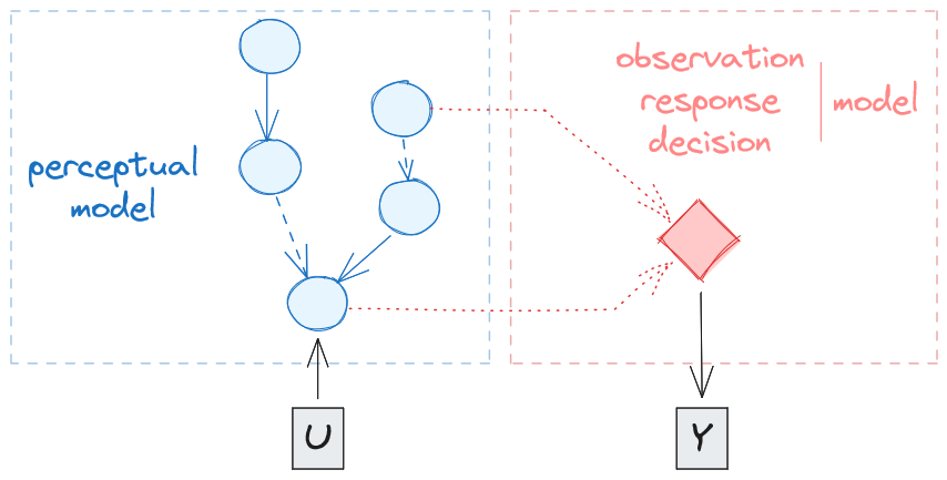
../_images/response_models.png — Fig. 5 **The Perceptual model and the Response model of a Hierarchical Gaussian Filter (HGF)**. The left panel represents the Perceptual model. The beliefs that the agent holds on state of the world are updated in the probabilistic network (blue circles) as the agent makes new observations (often noted \(u\), e.g. the association between a stimulus and an outcome at time \(t\)). Using these beliefs, the Response model (right panel) selects which decision/action \(y\) to perform. Critically here, the Response model only operates one-way (i.e. taking beliefs to generate action), but the actions are not modulating the way beliefs are updated (the model does not perform active inference - this point is, however, an active line of researches and new iterations of the model will try to *fusion* the two branch using active inference principles).#

Creating a new response function: the binary surprise#

To illustrate the creation of new response functions, we are going to use the same binary input vector from the decision task described in [Iglesias et al., 2021].

u, _ = load_data("binary")

For the sake of example here, we will consider that the participant underwent a one-armed bandit task, which consisted of the presentations of two stimuli (\(S_0\) and \(S_1\)) that could be associated with two types of outcomes (\(O_{+}\) and \(O_{-}\)). On each trial, the participant was presented with the two stimuli, chose one of them and get an outcome. The underlying contingencies of stimuli associated with positive outcomes are changing over time, in a way that can be more or less volatile. The Perceptual model tries to track these contingencies by observing the previous associations. We have already been using this Perceptual model model before in the tutorial on the binary HGF (The binary Hierarchical Gaussian Filter). Here the input data \(u\) is the observed association between e.g. \(S_0\) and \(O_{+}\). In order to incorporate a Response model on top of that, we need first to define:

a range of possible actions \(y\). In this case, the participant has only two alternatives so \(y\) can be either 0 or 1.
a Decision rule stating how the agent selects between the two actions given the beliefs of the probabilistic network at time \(t\). In this situation, it is trivial to write such a decision function and generate actions as new inputs are coming in, for simulation purposes for example. We start by setting a Perceptual model (i.e. a network of probabilistic nodes updated by observations). Here this is a standard two-level binary HGF, and the inputs are the binary observations (the association between one of the stimuli and the positive reward).

agent = HGF(
    n_levels=2,
    model_type="binary",
    initial_mean={"1": .0, "2": .5},
    initial_precision={"1": .0, "2": 1e4},
    tonic_volatility={"2": -4.0},
).input_data(input_data=u)

This perceptual model has observed the input sequence, meaning that we now have beliefs trajectories for all nodes in the network. The beliefs are stored in the variable node_trajectories in the model class, but can also be exported to Pandas using the to_pandas method like:

agent.to_pandas().head()

	time_steps	time	x_0_expected_mean	x_0_expected_precision	x_0_mean	x_0_precision	x_1_expected_mean	x_1_expected_precision	x_1_mean	x_1_precision	x_0_surprise	x_1_surprise	total_surprise
0	1.0	1.0	0.622459	0.235004	1.0	0.235004	0.500000	54.301674	0.506923	54.536678	0.474077	-1.077038	-0.602961
1	1.0	2.0	0.624085	0.234603	1.0	0.234603	0.506923	27.283697	0.520583	27.518301	0.471469	-0.731660	-0.260191
2	1.0	3.0	0.627284	0.233799	1.0	0.233799	0.520583	18.296556	0.540697	18.530355	0.466356	-0.530717	-0.064361
3	1.0	4.0	0.631975	0.232583	1.0	0.232583	0.540697	13.834867	0.566859	14.067450	0.458906	-0.389923	0.068983
4	1.0	5.0	0.638038	0.230946	0.0	0.230946	0.566859	11.185465	0.510971	11.416410	1.016216	-0.270900	0.745316

Creating the decision rule#

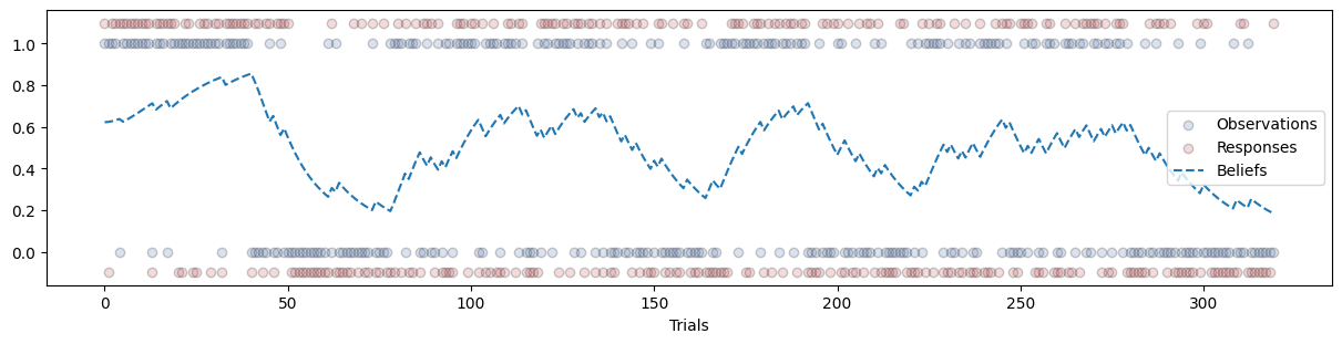
The next step is to use these beliefs to generate the corresponding decisions at each time point. We can work on the simplest Decision rule, which is probably to use the expected value of the first level a time \(t\) to sample from a binomial distribution and generate a binary decision. Intuitively, this just means that the agent is more likely to select a given stimulus when the beliefs that is is associated with a positive outcome are close to 1.0.

# a simple decision rule using the first level of the HGF
np.random.seed(1)
responses = np.random.binomial(p=agent.node_trajectories[0]["expected_mean"], n=1)

This gives us a binary vector of responses \(y\) that can be related to observations and underlying beliefs.

Text(0.5, 0, 'Trials')

../_images/be76219f96a1002af0f189b6276a6c1f7aa2a255fcb05dfb42aae689f21aef41.png

We now have the two ingredients required to create a response model:

the vector observations (\(u\)) that encode the current association between the stimuli and the outcomes.
the vector responses (\(y\)) that encode the inferred association by the participant, using the expected value at time \(t\) at the first level.

Note

We started by simulation the responses from an agent for the sake of demonstration and parameter recovery, but in the context of an experiment, the user already has access to the vectors \(y\) and \(u\) and could start from her.

Creating a new response function#

Let’s now consider that the two vectors of observations \(u\) and responses \(y\) were obtained from a real participant undergoing a real experiment. In this situation, we assume that this participant internally used a Perceptual model and a Decision rule that might resemble what we defined previously, and we want to infer what are the most likely values for critical parameters in the model (e.g. the evolution rate \(\omega_2\)). To do so, we are going to use our dataset (both \(u\) and \(y\)), and try many models. We are going to fix the values of all HGF parameters to reasonable estimates (here, using the exact same values as in the simulation), except for \(\omega_2\). For this last parameter, we will assume a prior set at \(\mathcal{N}(-2.0, 2.0)\). The idea is that we want to sample many \(\omega_2\) values from this distribution and see if the model is performing better with some values.

But here, we need a clear definition of what this means to perform better for a given model. And this is exactly what a Response model does, it is a way for us to evaluate how likely the behaviours \(y\) for a given Perceptual model, and assuming that the participants use this specific Decision rule. In pyhgf, this step is performed by creating the corresponding Response function, which is the Python function that will return the surprise \(S\) of getting these behaviours from the participant under this decision rule.

Hint

What is a response function? Most of the work around HGFs consists in creating and adapting Response model to work with a given experimental design. There is no limit in terms of what can be used as a Response model, provided that the Perceptual model and the Decision rule are clearly defined.

In pyhgf, the Perceptual model is the probabilistic network created with the main pyhgf.model.HGF and pyhgf.distribution.HGFDistribution classes. The Response model is something that is implicitly defined when we create the Response function, a Python function that computes the negative of the log-likelihood of the actions given the perceptual model. This Response function can be passed as an argument to the main classes using the keywords arguments response_function, response_function_inputs and response_function_parameters. The response_function can be any callable that returns the surprise \(S\) of observing action \(y\) given this model, and the Decision rule. The response_function_inputs are the additional data to the response function (optional) while response_function_parameters are the additional parameters (optional). The response_function_inputs is where the actions \(y\) should be provided.

Important

A response function should not return the actions given perceptual inputs \(y | u\) (this is what the Decision rule does), but the surprise \(S\) associated with the observation of actions given the perceptual inputs \(S(y | u)\), which is defined by:

\[ \begin{align} S(y | u) = -\log[Pr(y | u)] \end{align} \]

If you are already familiar with using HGFs in the Julia equivalent of pyhgf, you probably noted that the toolbox is split into a perceptual package HierarchicalGaussianFiltering.jl and a response package ActionModels.jl. This was made to make the difference between the two parts of the HGF clear and be explicit that you can use a perceptual model without any action model. In pyhgf however, everything happens in the same package, the response function is merely an optional, additional argument that can be passed to describe how surprise is computed.

Therefore, we want a Response function that returns the surprise for observing the response \(y\), which is:

\[\begin{split} \begin{align} surprise | y & = \sum_{t=1}^{t} - \log(p(y^t | \hat{\mu}_1)) \\ & = \sum_{t=1}^{t} - \log(\hat{\mu}_1^y(1 - \hat{\mu}_1)^{1-y}) \\ \end{align} \end{split}\]

We can write such a response function in Python as:

def response_function(hgf, response_function_inputs, response_function_parameters=None):
    """A simple response function returning the binary surprise."""

    # response_function_parameters can be used to parametrize the response function (e.g. inverse temperature)
    # ...<

    # the expected values at the first level of the HGF
    beliefs = hgf.node_trajectories[0]["expected_mean"]

    # get the decision from the inputs to the response function
    return jnp.sum(jnp.where(response_function_inputs, -jnp.log(beliefs), -jnp.log(1.0 - beliefs)))

This function takes the expected probability from the binary node and uses it to predict the participant’s decision. The surprise is computed using the binary surprise (see pyhgf.update.binary.binary_surprise()). This corresponds to the standard binary softmax response function that is also accessible from the pyhgf.response.binary_softmax() function.

Note

Note here that our Response function has a structure that is the standard way to write response functions in pyhgf, that is with two input arguments:

the HGF model on which the response function applies (i.e. the Perceptual model)
the additional parameters provided to the response function. This can include additional parameters that can be part of the equation of the model, or the input data used by this model. We then provide the response vector (\(y\)) here.

Note that the operation inside the function should be compatible with JAX’s core transformations.

# return the overall surprise
response_function(hgf=agent, response_function_inputs=responses)

Array(205.87854, dtype=float32)

We now have a response function that returns the surprise associated with the observation of the agent’s action. Conveniently, this is by definition the negative of the log-likelihood of our model, which means that we can easily interface this with other Python packages used for optimisation and Bayesian inference like PyMC or BlackJAX. We use the surprise as a default output, however, as this metric is more commonly used in computational psychiatry and is more easily connected to psychological functioning.

Recovering HGF parameters from the observed behaviors#

Now that we have created our Response function, and that we made sure it complies with the standard ways of writing responses functions (see above), we can use it to perform inference over the most likely values of some parameters. We know that the agent used to simulate behaviour had an evolution rate set at -4.0. In the code below, we create a new HGF distribution using the same values, but setting the \(\omega_2\) parameter free so we can estimate the most likely value, given the observed behaviours.

hgf_logp_op = HGFDistribution(
    n_levels=2,
    model_type="binary",
    input_data=u[jnp.newaxis, :],
    response_function=response_function,
    response_function_inputs=responses[jnp.newaxis, :]
)

Note

The response function that we created above is passed as an argument directly to the HGF distribution, together with the additional parameters. The additional parameters should be a list of tuples that has the same length as the number of models created.

with pm.Model() as sigmoid_hgf:

    # prior over the evolution rate at the second level
    tonic_volatility_2 = pm.Normal("tonic_volatility_2", -2.0, 2.0)

    # the main HGF distribution
    pm.Potential("hgf_loglike", hgf_logp_op(tonic_volatility_2=tonic_volatility_2))

with sigmoid_hgf:
    sigmoid_hgf_idata = pm.sample(chains=2, cores=1)

Auto-assigning NUTS sampler...

Initializing NUTS using jitter+adapt_diag...

Sequential sampling (2 chains in 1 job)

NUTS: [tonic_volatility_2]

Sampling 2 chains for 1_000 tune and 1_000 draw iterations (2_000 + 2_000 draws total) took 6 seconds.

We recommend running at least 4 chains for robust computation of convergence diagnostics

az.plot_trace(sigmoid_hgf_idata, var_names=["tonic_volatility_2"]);
az.summary(sigmoid_hgf_idata, var_names=["tonic_volatility_2"])

	mean	sd	hdi_3%	hdi_97%	mcse_mean	mcse_sd	ess_bulk	ess_tail	r_hat
tonic_volatility_2	-3.953	0.504	-4.946	-3.084	0.017	0.012	937.0	1321.0	1.0

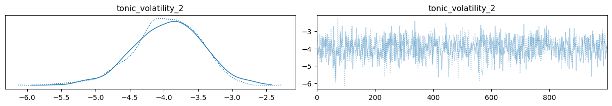
../_images/6cc16a2f8845a45e05387c434b81876830179c00ec7c2052457dafd3694edea8.png

The results above indicate that given the responses provided by the participant, the most likely values for the parameter \(\omega_2\) are between -4.9 and -3.1, with a mean at -3.9 (you can find slightly different values if you sample different actions from the decisions function). We can consider this as an excellent estimate given the sparsity of the data, and the complexity of the model.

Glossary#

Perceptual model#: The perceptual model of a Hierarchical Gaussian Filter traditionally refers to the branch receiving observations \(u\) about states of the world and that performs the updating of beliefs about these states. By generalisation, the perceptual model is any probabilistic network that can be created in pyhgf, receiving an arbitrary number of inputs. An HGF that only consists of a perceptual model will act as a Bayesian filter.
Response model#: The response model of a Hierarchical Gaussian filter refers to the branch that uses the beliefs about the state of the world to generate actions using the Decision rule. This branch is also sometimes referred to as the decision model or the observation model, depending on the fields. Critically, this part of the model can return the surprise (\(-\log[Pr(x)]\)) associated with the observations (here, the observations include the inputs \(u\) of the probabilistic network, but will also include the responses of the participant \(y\) if there are some).
Decision rule#: The decision rule is a function stating how the agent selects among all possible actions, given the state of the beliefs in the perceptual model, and optionally additional parameters. Programmatically, this is a Python function taking a perceptual model as input (i.e. an instance of the HGF class), and returning a sequence of actions. This can be used for simulation. The decision rule should be clearly defined in order to write the Response function.
Response function#: The response function is a term that we use specifically for this package (pyhgf). It refers to the Python function that, using a given HGF model and optional parameter, returns the surprise associated with the observed actions.

System configuration#

%load_ext watermark
%watermark -n -u -v -iv -w -p pyhgf,jax,jaxlib

Last updated: Sun Oct 13 2024

Python implementation: CPython
Python version       : 3.12.7
IPython version      : 8.28.0

pyhgf : 0.2.0
jax   : 0.4.31
jaxlib: 0.4.31

IPython   : 8.28.0
matplotlib: 3.9.2
numpy     : 1.26.0
arviz     : 0.20.0
jax       : 0.4.31
pymc      : 5.17.0
sys       : 3.12.7 (main, Oct  1 2024, 15:17:55) [GCC 11.4.0]
pyhgf     : 0.2.0

Watermark: 2.5.0