pyhgf.plots.plot_trajectories

pyhgf.plots.plot_trajectories(network: Network, ci: bool = True, show_surprise: bool = True, show_posterior: bool = False, show_total_surprise: bool = False, figsize: Tuple[int, int] = (18, 9), axs: List | Axes | None = None) → Axes

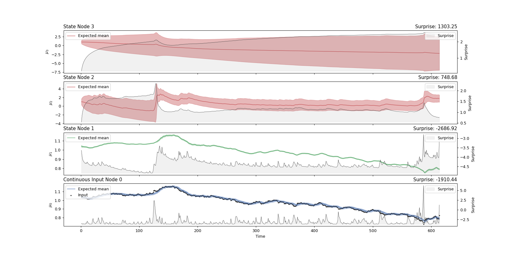
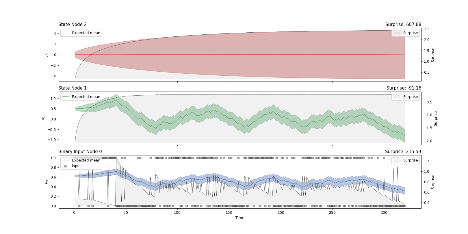
Plot the trajectories of the nodes’ sufficient statistics and surprise.

This function will plot the expected mean and precision (converted into standard deviation) and the surprise at each level of the node structure.

Parameters:

network

An instance of the main Network class.

ci

Show the uncertainty around the values estimates (standard deviation).

show_surprise

If True plot each node’s surprise together with sufficient statistics. If False, only the input node’s surprise is depicted.

show_posterior

If True, plot the posterior mean and precision on the top of expected mean and precision. Defaults to False.

show_total_surprise

If True, plot the sum of surprises across all nodes in the bottom panel. Defaults to False.

figsize

The width and height of the figure. Defaults to (18, 9) for a two-level model, or to (18, 12) for a three-level model.

axs

A list of Matplotlib axes instances where to draw the trajectories. This should correspond to the number of nodes in the structure. The default is None (create a new figure).

Returns:

axs

The Matplotlib axes instances where to plot the trajectories.

Examples

Visualization of nodes’ trajectories from a three-level continuous HGF model.

from pyhgf import load_data
from pyhgf.model import HGF

# Set up standard 3-level HGF for continuous inputs
hgf = HGF(
    n_levels=3,
    model_type="continuous",
    initial_mean={"1": 1.04, "2": 1.0, "3": 1.0},
    initial_precision={"1": 1e4, "2": 1e1, "3": 1e1},
    tonic_volatility={"1": -13.0, "2": -2.0, "3": -2.0},
    tonic_drift={"1": 0.0, "2": 0.0, "3": 0.0},
    volatility_coupling={"1": 1.0, "2": 1.0},
)

# Read USD-CHF data
timeserie = load_data("continuous")

# Feed input
hgf.input_data(input_data=timeserie)

# Plot
hgf.plot_trajectories();

Visualization of nodes’ trajectories from a three-level binary HGF model.

from pyhgf import load_data
from pyhgf.model import HGF
import jax.numpy as jnp

# Read binary input
u, _ = load_data("binary")

three_levels_hgf = HGF(
    n_levels=3,
    model_type="binary",
    initial_mean={"1": .0, "2": .5, "3": 0.},
    initial_precision={"1": .0, "2": 1e4, "3": 1e1},
    tonic_volatility={"1": None, "2": -6.0, "3": -2.0},
    tonic_drift={"1": None, "2": 0.0, "3": 0.0},
    volatility_coupling={"1": None, "2": 1.0},
    eta0=0.0,
    eta1=1.0,
    binary_precision = jnp.inf,
)

# Feed input
three_levels_hgf = three_levels_hgf.input_data(u)

# Plot
three_levels_hgf.plot_trajectories();